Building Objects

Introduction

ArtMatic Voyager uses a unique approach to 3D object modelling and rendering called Distance Field Ray Marching, or DFRM. This guide explains how to create and modify 3D objects represented by distance fields, or DF objects, and provides practical guidelines for working with them. The technical background may also help you understand the reasoning behind those guidelines and develop your own techniques.

DFRM Concept

ArtMatic Voyager uses a technique called ray marching to render images. Ray marching samples points along a ray between the observer and the scene until it finds where that ray intersects an object or terrain. This can be slow, because the scene may need to be sampled many times before the intersection is found. Ray marching is useful when the mathematics that describe the object are too complex for direct analytical intersection, such as an entire procedural planet in ArtMatic Voyager.

Distance fields make this process much more efficient. Instead of advancing along a ray by small fixed steps, ArtMatic Voyager can use the distance field itself to estimate how far the ray is from the surface. This lets the renderer take larger, safer steps and converge on the surface more quickly.

A distance field is a scalar field whose value gives a good, or exact, estimate of the distance to a surface.

The distance field does not have to be mathematically exact, but the more accurate the estimate, the faster the renderer can converge. If the estimate is too large, the ray may overshoot the surface and miss the object. Underestimation does not usually prevent convergence, but it makes the process slower.

A distance field function takes space or plane coordinates, and calculates an estimate of the distance from that point to the object surface. The object surface is where the distance is zero: the “zero crossing” of the field. A value greater than zero indicates a point inside the object, with the field value indicating the distance from the surface. A value less than zero indicates a point outside the object. ArtMatic’s Geographic CLUT colour shader is useful for visualising distance fields, because its colours indicate distances.

A distance field can be 2D or even 1D. A 1D distance field is simply X, Y, or Z, provided it is unscaled.

Tip

For example, you can use –Y directly to create an infinite flat DF ground plane where Y == 0 defines the surface.

The simplest 3D distance field is a sphere. Remarkably, the sphere equation is also its own distance field equation.

The field is described as

R – sqrt(x^2 + y^2 + z^2), or R - length(x, y, z), where length is the Euclidean distance.

This comes from the sphere equation x^2 + y^2 + z^2 = R, where R is the radius of the sphere. The minus sign adjusts the field values so that the field is negative outside the sphere and positive inside.

With a sphere, convergence can happen in a single step because R - length(x, y, z) gives the exact distance to the surface. The field exists everywhere in space, which makes DF objects non-local, unlike classical polygonal descriptions.

A distance field can be seen as a special kind of scalar field. Scalar fields are non-directional, unlike vector fields, and non-local. Because the field exists everywhere in space, the object information extends far beyond the object’s visible boundaries. This property is useful: a simple offset of the field value can expand or shrink the object.

DF fields can be manipulated in many ways that are impossible, or very difficult, with polygonal descriptions:

• DF fields can be blended or morphed together.
• DF fields can be distorted by space-distortion functions.
• DF fields can be combined using Boolean operators.
• DF fields can be used as the input coordinates for another DF field calculation.

DFRM is useful not only because it is computationally efficient, but because simple operations can create complex and interesting shapes. Animating these transformations can produce object morphs that would be very difficult to create with more traditional 3D tools.

DF fields provide a unified representation for very different types of objects:

• a tree,
• a fractal,
• a building,
• a sphere.

This representation is non-local and independent of any particular topology, which makes it relatively easy to morph and combine very different objects. As a result, DF objects make efficient and flexible 3D modelling techniques possible, and ArtMatic Engine provides hundreds of functions designed for DF modelling.

ArtMatic 3D DF Objects

3D DF objects are created using ArtMatic Designer. Creating and modifying them requires a fairly good understanding of ArtMatic Structure Trees. Many pre-existing DF primitives are available in ArtMatic Engine to provide basic DF building blocks that you can combine using Boolean functions. For the most part, you will use built-in ArtMatic components that generate distance fields and combine them, using the guidelines provided later, to create complex objects. Although advanced users can create their own distance fields, it is unlikely that you will ever need to create a distance field from scratch.

ArtMatic Trees need certain properties to work as DF objects. Any 2D or 3D scalar function can be interpreted as a distance field, (as long as the field value provides a good distance approximation to the function zero crossing, or surface). 3D object Trees need to be 3D, which means they use the X, Y, and Z global inputs. The field has to be negative outside the object surface and positive inside. All functions that are clamped to zero, positive only, cannot be used as DF-generating functions.

A DF object is not necessarily bounded and small. You can have one DF object describing an entire city or forest. Using a Compiled Tree, there are virtually no limits to the number of functions and complexity of geometry you can have in a single DF object instance.

Scaling & Size

The scaling of a DF object is always absolute, and the overall size can be set within Voyager as a percentage in the Object Inspector. Sometimes, however, it is necessary to scale DF elements within the ArtMatic Tree when merging various shapes or building fractals. In general, most DF building blocks have a Radius or Scale parameter that sets the element size directly.

Changing object size is generally done by adding an offset to the distance field value rather than by scaling space. If you must scale space, it is necessary to compensate by inverse-scaling the field value to maintain a proper DF estimate. Take the case of a sphere. If X, Y, and Z are scaled by 4, the distance estimate becomes four times larger than it should be. Scaling down by 1/4 corrects the error. This is equivalent to lowering the radius by subtracting an offset from the field itself.

A couple of special components, S-space scaling components, keep track of scaling automatically so that the field can be adjusted at the end of the Tree with the proper inverse value. 44 space transforms provide many operators that keep track of the S-scale, allowing you to build fascinating DF-based volumetric fractals.

Rotation and mirroring functions can be used safely, as they do not change the space scaling and keep the distance field accurate.

Positions

Voyager provides many sliders and ways to position the entire DF object in the scene. When an ArtMatic Tree mixes several DF objects, it is often necessary to position the objects relatively within the Tree. A simple space translation does not modify the DF field accuracy and is safe to use. The 1D Offset component, 3D Offset component, and any vector offset functions can all be used to move various parts. A translation is a simple addition of a constant value to a space coordinate. If the relative displacement is needed in only one dimension, it is efficient to use the 1:3 Add vector function.

To animate the object position, use ArtMatic keyframes with varying offset Tile parameters, or more complex motion functions connected to global time input W.

Object Colour

To associate a colour with a DF field, you will typically use the RGBA stream format, with A holding the distance estimation data. A constant colour Tile can provide the RGB data if the object has a single colour and no texture. Advanced users will build a colour texture function to feed the RGB associated with the object. As with terrain textures, the object texture is computed after the intersection phase, and you can optimise rendering speed by separating texture computation from object distance-field computation. In that case, put all Tiles used to compute the colour texture in a Compiled Tree and set the Compiled Tree to Evaluate Only For Colors. Any Tile with the Evaluate Only For Colors option set will not be computed during the intersection phase. See Rendering Passes in ArtMatic Surfaces. The colour texture function will often be a 3:3 Tile that gets its input from incoming space and outputs RGB data.

In more recent versions, many DF RGBA functions output both a DF field and a colour. These can be used to carve a DF field and provide colour to the object at the same time. When all RGBA channels are used by the same component, it is no longer possible to use the Evaluate Only For Colors option, because the component also affects the geometry.

Specific Boolean operators were added in Engine 8.5 to simplify DF object texturing.

Previewing in ArtMatic

Since ArtMatic Designer has only a 2D view, you will see a slice of the field. 3:3 space transforms, such as 3D Spaces# ArtMatic top view, are handy for seeing a top-view map of the field, even if the Voyager rendering shows the object standing. You may also use a 3D rotation Tile and set up a group of views using ArtMatic keyframes to ‘look’ at the object slice from different directions.

When creating DFRM objects in ArtMatic, it is often useful to switch between shaders. The Geographic CLUT, in particular, is great for visualising the distance field and making sure it is correct. Geographic CLUT makes it easy to see if there are anomalies caused by too much scaling or distortion. For all objects, there should be an orderly and reasonable transition as one moves away from the surface or into the object’s interior. The negative region outside the object is shaded in blue, while the interior is shaded with a geographic colour ramp according to the distance estimate. To see a preview of a texture function, switch the ArtMatic shader to RGB Density to get a slice of the colour texture. Regions outside the object are treated as transparent.

The most efficient way to model in ArtMatic is to have Voyager running in the background and allow ArtMatic to send data to Voyager using the Link button. In that case, you will see a preview window of the 3D Voyager rendering while working in ArtMatic Designer. You can then fine-tune many parameters while seeing the 3D result interactively.

Note: When using Voyager and Designer concurrently, make sure that ArtMatic Designer is launched before you click an “Edit in ArtMatic” button. This ensures the correct version is used.

Design Guidelines

• Don’t scale the space
  If you must, do it only with the 3:4 S-Space Scale function, and don’t forget to divide the DF field by the S value at the end. In general, growing DF objects is done more efficiently by adding to or subtracting from the field itself. A simple offset connected to a DF output will thicken or thin the field.

• Don’t distort space too much
  If you must, compensate by scaling down the DF field. When using arbitrary noise functions for displacement, make sure not to use amplitudes that are too large. If the amplitude is too large, the displacement may be so large that DFRM will not converge or will miss certain areas, resulting in artefacts. The solution is to reduce the amplitude parameter or add a filter to the output to reduce the values.

• Don’t overblend with non-DF functions
  Many interesting functions for terrain design are available in ArtMatic Engine. These functions, even without being true DF estimates, can still be used to add textures or deformations to DF fields by blending them with the DF function. As with scaling, do this sparingly, and if convergence is affected, reduce the amplitude of the final DF value.

• Don’t use additions
  Use rotate interpolation or linear interpolation instead of +. Interpolations will make the DF estimate slightly undershoot, while addition will make it overshoot. Undershooting is fine: with a distance estimation that is below the real distance, you will always converge to the solution, just a bit more slowly. Overshooting is bad: it can produce rendering artefacts and, in the most catastrophic situation, the object may simply disappear.

• Use logical operators to combine DF fields. Logical operators like MIN and MAX do not scale or damage field accuracy, so they are perfect for mixing various DF objects. Many logical-operator components are provided for scalar and RGBA DF fields by ArtMatic Engine.

  • S:P Logic & Profiles
  • 21 Logic tools #
  • 24 Packed Logic #
  • 34 Packed Logic #

  Examples of logical operators are located in Voyager Examples/Components/Logic tools.

• Use Compiled Trees (CT) and the divide-and-conquer method
  For complex modelling, try to break the problem into smaller parts. You can model and test each part separately and make them into a CT, usually of the form 3 in / 1 out, with a packed RGBA output so that the object contains its own texture as well as its geometry. When all is set, you can copy and paste the CT into the bigger project.

  CTs can be nested, so you can always replace one branch with a collection of functions packed into a CT. Think of a CT as a logical group of objects. A good practice is to place a 3:3 translate on top of each CT so that you can move each part relative to others. Everything connected to a particular space transform will share its coordinate system and be moved with it. Transforms included below it will be relative to the transform above, so you can design complex articulated motions while keeping track of the flow of transforms and their dependencies.

  Imagine, for example, a rotating articulated robot arm placed on a wagon on a rail. The logic of what is needed, and what should depend on what, determines the structure and flow of information, and therefore the structure of the Tree. The wagon and arm move together: they are two branches connected to the same space. The arm has various articulated parts: put them in a CT with a rotation on top, as the entire thing rotates. Each arm part can be another CT connected in cascade so that the hand moves correctly when the first part rotates.

  It is always good to take some time to clearly understand what is needed and break the problem into smaller chunks. Start with simple 3D objects to get the structure and behaviour right. Then you can refine them separately in other Trees and replace the draft version with the final model using copy/paste of the CT.

  Designing a generic multi-CT model is a huge time saver, as the same structure can easily be changed to make many models. The examples provided in the Voyager 1.5 installation — Path Profiles Church, Path Profiles TwinTowers, and Path Profiles Rect4D.vy — demonstrate this.

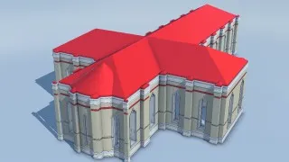
Example of a generic CT-designed model Tree: Voyager Examples/DF Modelling/Architecture Classics/Path Profiles Church.

DF Modelling Techniques

Many times, it is simpler to build a 3D object using 2D DF profiles like the ones provided by 21 Profile Shapes # or 21 DF Curves #.

A 2D DF profile is simply a DF field defined in only 2 dimensions; it is infinite in the undefined dimension. For example, a 2D DF disc connected to (x, z) renders as an infinite column in Voyager because Y is not specified.

Examples of basic modelling techniques are located in Voyager Examples/DF Modelling/Basic techniques.

The most useful techniques for working with 2D profiles are:

Intersection

You can intersect two 2D DF fields defined in different planes to create a 3D object. Think of a 2D DF field as a “profile path” where the zero crossing of the field defines the path shape. Used directly in 3D, these profiles are infinite in the other axis, typically Z if the 2D DF component is connected to (x, y), or Y if the 2D DF is connected to (x, z).

By intersecting an (x, y) profile with an (x, z) profile, you ensure the object is bounded in all dimensions. The result is a 3D object that looks like profile A in one direction and profile B in the perpendicular direction. The intersection is typically performed using Boolean, or logical, operators like 21 Logic tools # or S:P Logic & Profiles, but for a basic intersection, a simple Minimum function will work.

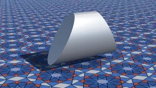
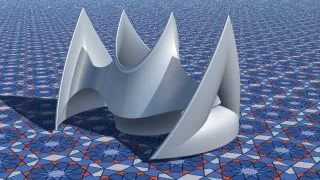
A 2D triangle in (x, y) intersects with a 2D ellipse in (y, z).

The intersection can itself add details to the geometry using various flavours of the Boolean operator. “Edged intersect”, for example, will add edges at the intersection.

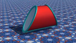
A 2D triangle in (x, y) edged-intersects with a 2D red ellipse in (y, z).

---

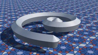
Sweeps

As DF fields can be used as the input coordinates for another field calculation, it is possible to use a 2D DF field as an input, X, Y, or Z, for another DF function, either 2D or 3D. This basically ‘sweeps’ object B along the profile of object A. For example, to get a torus, sweep a disc in (x, y) along a circular path defined by a disc profile in (x, z). Sweeping any profile with a disc will create a revolution object, such as a glass or bottle.

Usually, you will connect a 2D profile directly to one coordinate input of another 2D profile. Another way is to use the 3:2 Revolution & Sweeps component, which provides many paths for sweeps.

When 2D UV coordinates are needed, you may also use the 3:4 uvid Sweep Volumes component, which performs sweeps internally and returns UV as well as the DF field itself.

A 2D pentagon (2:1 Profile Shapes) sweeps along an Archimedes spiral path (2:1 DF Curves).

---

Cross Sweep

A cross-sweep is achieved when a 2D profile is connected to two other 2D profiles, one fed into the X input and the other into the Y input.

Quite complex models can be achieved that way.

A 2D Triangle and a 2D disk (2:1 Profile Shapes) feed coordinates of a 2:1 DF Curves object.

There are many ways to work with 3D DF fields, and the techniques below can all be combined to achieve quite complex geometry.

---

Intersection, Union, etc.

Most of the time, you will build complex 3D objects by mixing various 3D DF fields, using Boolean, or logical, operators like 2:1 Logic tools.

Many examples of logical-operator usage are located in Voyager Examples/Components/Logic tools.

---

Morphing Fields

Use the Morph components to make a morphed union of 2 objects. For scalar fields, you can use the Math tools | Morph function. To morph 2 coloured DF objects, use the 2:4 Tile Packed Morph.

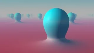
A cyan sphere array morphed with an infinite red DF plane.

---

Sweeps & Cross-sweeps

Sweeps can also work between 3D and 2D DF objects. You ‘sweep’ a 2D DF profile along a 3D DF field by feeding the 3D object field to one of the 2D DF profile coordinates.

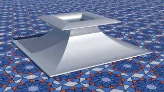
A 2D arc curve sweep along a four-sided 3D pyramid.

It is also possible to sweep a 2D profile along the intersection of two 3D DF volumes. In that case, the 2D profile traces the shape of the intersection contours.

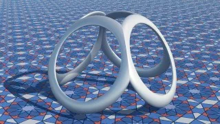
A 2D disc sweep along the intersection of a sphere and a four-sided pyramid.

---

Space Deformation

A very efficient way to shape the DF object is to add a space-distortion function to modify the incoming space. Mirroring and rotations are very often used to force the object to be symmetrical or to have various numbers of rotational symmetries.

3D mirroring and rotations are as follows:

• 3D Plane Mirror,
• 3D Mirrors & Rotates,
• 3D Mirrors & Offset

A 3D fractal displacement like 3D Fractal displace will completely change the look of a simple sphere. Some displacement functions are specifically designed to deform DF fields, such as 3D Distorts & Bend #.

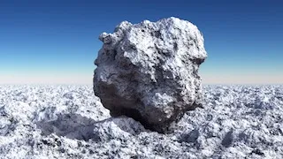
A DF sphere and ground with 3D space displaced by 3D Fractal displace.

---

Displace the Field Value

To add a bump texture or small details, you can simply add a small amount of a 3D noise function to the field. A number of 3D DF noise and 3D DF pattern functions are available in ArtMatic Engine to add textures at the geometry level. For small details, almost every ArtMatic function can be used to modulate the DF field.

Examples of 3D noise added to a sphere:

• 3D Ridged Fractal,
• 3D Fractal Bubbles

---

Instantiation by Space Manipulation

The most efficient way to duplicate and instantiate objects is to manipulate space so that a single object appears in many places at once. A simple 1D Modulo function will repeat the object infinitely along one axis, for example. You may use a Voronoi diagram, 2D or 3D, to partition space into many cells, each having its own coordinates. ArtMatic Engine provides many components that create instances by tiling or partitioning space:

• 3D Repeats and Tile,
• Jitter Spherical,
• Jitter Axial,
• Motion Cluster,
• 3D Motion Path render

The difficulty with this technique is that the DF field has to be well centred and relatively far from the space cell boundaries, where space coordinates suddenly become discontinuous and jump to totally unrelated values. To maintain an accurate distance estimate and avoid overshooting, you can clamp the DF value when using these so that it does not go below a fixed value.

When the tiling is regular and space is symmetrical, the problem vanishes, as the space is coherent even at cell boundaries.

---

Carving

A 3D pattern or noise component can provide details to any 3D volume using S:P Logic & Profiles displacement functions like ‘Displace’, ‘Chisel displace’, and ‘Circle displace’. They carve the volume along the contours defined by the zero crossings of the 3D volumetric pattern. You can also carve an object using intersection or subtraction Booleans.

ArtMatic Engine 8.5 provides functions for carving a DF texture, including S:P Logic & Profiles Texture Intersect and Fuzzy Intersect. Fuzzy Intersect is also available in 24 Packed Logic #.

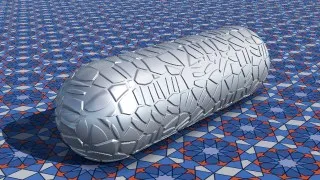
An elongated sphere (XYZ Shapes) carved with a Voronoi split pattern (3D Bubble & skins).

In ArtMatic Engine 8.5 and the corresponding Voyager 1.5 release, a large number of DF colour textures and patterns were added. A simple DF surface carved with a complex RGBA DF pattern can yield rich results, because the carving texture provides both colour and geometry.

Jittered City shapes colour-carved with the “conics elements” RGBA DF pattern.

---

Shading DF Objects

Textured or not, Voyager provides several rendering and shading options for DF objects. In general, you will use Opaque mode, but alternate modes provide:

• clouds and gases,
• fuzzy objects,
• light fields,
• transparent/translucent objects.

Examples are provided in Voyager Examples/Shading & Rendering/ folders.

Volumetric Opaque

This mode shades the 3D object as an opaque solid object. If the ArtMatic system has only a single output value, the output defines the object’s shape, and the colour is white, although the apparent colour can be changed using the object’s specular/reflection properties. If the ArtMatic system provides RGBA output, the alpha channel defines the object’s shape and the RGB outputs provide the object’s colours.

ArtMatic extra outputs, or X-outs, are used if specified in the Voyager settings. Volumetric Opaque can be used for a mind-boggling variety of objects and features.

---

Volumetric Light

This mode shades the DF field as a volumetric light density field by accumulating colour/opacity values along the ray. It is suited to a wide range of luminous effects:

• fire,
• city lights,
• arrays of lights.

The occlusion slider determines how much light from the background is occluded by the object. The light density parameter scales the distance field interpreted as density values when inside the object.

You often need to adjust it when the light gets too saturated or too bright. This mode is slower than Volumetric Opaque, as the object, meaning its density field, needs to be scanned inside and out, whereas evaluation of an opaque object stops where the light rays meet the object’s exterior.

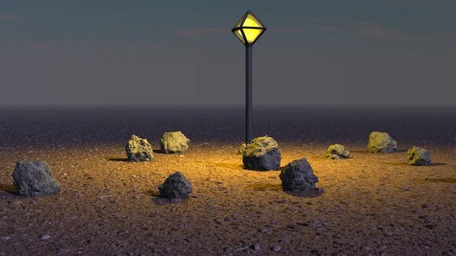
Volumetric Light objects can cast light. The light emission range parameter controls how far light is cast from the distance field centre. The light direction is taken from the normal of the DF field unless you use “Shade as Projector” mode, in which case the object centre becomes the source of light. Light cast with the DF normal may be physically impossible and won’t cast shadows, but it is nevertheless quite efficient for rendering multiple lights or complex light fields, such as city street lights. Alternatively, you may have an extra output defining the light direction vector. In that case, you can automate the X-out settings by using the letters ib at the end. The ‘b’-tagged X-out vector defines the light direction vector. In that case, the light field will cast shadows.

Examples: Voyager Examples/Shading & Rendering/DF lights fields

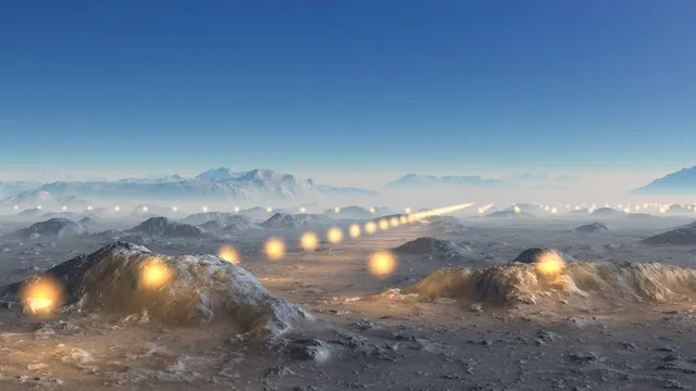
In the Desert Light Field example, you can see an array of lights casting light on the desert.

---

Jitter Opaque

This mode replicates an object throughout an environment with small variations so that the repetitions are not identical. Voyager essentially breaks up the environment into randomised cells and instantiates one copy of the object into each cell with a ‘jittered’, or randomised, centre and rotation. ArtMatic global A3 is sent a unique randomised value for each cell that can be used to randomise the object properties.

You can use this technique to create an entire forest from a single tree. If you use an ArtMatic system that uses a jittering component, make sure that the ArtMatic system’s jittering clip radius is smaller than Voyager’s jitter cell size, and keep the object small enough so it stays away from cell boundaries.

This may require some experimentation to find the correct parameter values. For greater control, you would usually use a jittering Tile within the ArtMatic Tree.

Learn more at Modelling Techniques: Instantiation by Space Manipulation.

---

Volumetric and Translucent

This shading variant of Opaque mode is dedicated to vegetation, such as leaves and plants. It adds light passing through the object and light scattered inside the object surface. The thickness of the object is important, as a thin object, such as a leaf, tends to be more translucent than a trunk.

The ‘Light Transmission’ and ‘Light Transmission Range’ parameters control how much light can travel through the medium and how deeply. ‘Light Transmission Range’ ranges from 0 to 200 metres. Light travelling inside the medium is coloured by the reflection colour and the object texture colour.

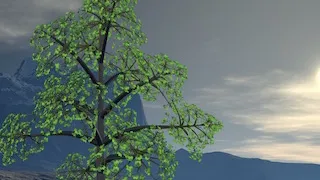
Backlit trees will still have light passing through the leaves in this mode.

---

Fractal Opaque

This mode is designed for fractal objects and objects with very rough surfaces, as it smooths the sub-pixel details that would otherwise make the image noisy, especially when far away.

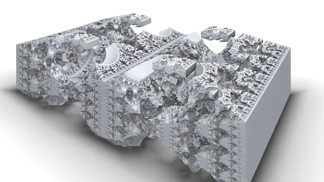
The global high-frequency limit and the Fractal Object Detail percentage % in the Preferences dialog further allow fine control over object details. Use this mode for fractal objects with very rough or infinitely thin structures like the MandelBulb, the MandelBox, and similar objects created with 32 3D Fractal sets.

---

Transparent (Surface)

This mode is suited to transparent objects like glass or windows. The object surface is treated as transparent, without internal volumetric shading or refraction calculations. Light colour is tinted as it passes through the object, much as it would be affected by tinted glass. The stained glass windows in the Opaque + Transparent example are treated as transparent surfaces. Notice how they project their colours on the ground and walls. Transparent mode does not generate new rays and is faster than Transmissive modes.

---

Transmissive (Surface)

Introduced in ArtMatic Voyager 1.2, “Transmissive” can render refracting material. Transmissive offers several air/medium indices of refraction with a single ray or multiple rays.

While a single ray gives physically inexact results for bounded objects, it is fast and can produce pleasing, less noisy results. A single ray is sufficient for water planes, for example, where there will not be an exit from the medium on the other side. With multiple-ray mode, it is possible to place the camera inside the object.

Surface mode only handles rays at the intersection and does not perform volumetric density estimation, unlike Transmissive (Volumetric) mode.

Specific parameters: Surface Shade and Tint Gain. Surface Shade controls how much the surface is shaded, balanced with light coming through the medium with refractions. When Surface Shade is at maximum, the object is completely opaque. Tint Gain controls how much light going through the medium is coloured by the object colour. Use strong values for stained glass, for example.

Transmissive (Surface) has the following options:

Material Type	Number of Rays	Index of Refraction
Helium	1 Ray	IOR = 1.025 Air = 1
Jelly	1 Ray	IOR = 1.125
Water	1 Ray	IOR = 1.333
Glass	1 Ray	IOR* = 1.52
Helium	Multi-Ray	N/A
Jelly	Multi-Ray	N/A
Water	Multi-Ray	N/A
Glass	Multi-Ray	N/A
Diamond	Multi-Ray	IOR = 2.417

Note

Multiple rays implementation. Note that ray number is limited to 4 in Good quality and 6 > in higher quality.

Examples are provided in Shading & Rendering/DF Special Shaders/.

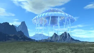
Transmissive jellyfish.

---

Transmissive (Volumetric)

This mode offers several air/medium indices of refraction with a single ray or multiple rays. Unlike Surface mode, it can also accumulate opacity along the ray for volumetric density evaluation, with the parameter ‘Opacity Gain’ controlling volumetric density. The volumetric density shading can be a simple diffuse shader, in shaded variants, or just take the object colour unshaded, in unshaded variants. This corresponds to the previous versions’ “Self-Illum mode” when ambient level is above zero.

Specific parameters: Surface Shade and ‘Opacity Gain’.

Transmissive (Volumetric) mode has the following options:

Material Type	Number of Rays	Shading
Helium	1-Ray	Unshaded
Jelly	1-Ray	Unshaded
Water	1-Ray	Unshaded
Glass	1-Ray	Unshaded
Helium	1-Ray	Unshaded
Jelly	1-Ray	Unshaded
Water	1-Ray	Unshaded
Glass	1-Ray	Unshaded
Diamond	1-Ray	Unshaded
Helium	Multi-Ray	Unshaded
Jelly	Multi-Ray	Unshaded
Water	Multi-Ray	Unshaded
Glass	Multi-Ray	Unshaded
Diamond	Multi-Ray	Unshaded
Helium	Multi-Ray	Shaded
Jelly	Multi-Ray	Shaded
Water	Multi-Ray	Shaded
Glass	Multi-Ray	Shaded
Diamond	Multi-Ray	Shaded

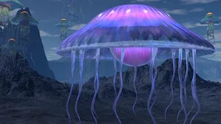
Transmissive self-illum jellyfish.

---

Fuzzy Loose

This is a faster version of ‘Fuzzy’ mode that renders less accurately than ‘Fuzzy’ by sampling the volume much more sparsely. Use this mode if the other is too slow for fast previewing.

Fuzzy

Only the volumetric interior is rendered and shaded by accumulation, and there is no surface shading. Specular is off in this case. ‘Fuzzy’ shading mode can be used for fuzzy objects and even plants.

Gas and Clouds

In this mode, density objects are shaded like clouds. This provides an alternate, more flexible and controllable solution than volumetric clouds. With Gas and Clouds, you can make smoke, steam, fog, clouds, and even vegetation for an impressionistic approximation when seen from afar. Examples: Voyager Examples/Shading & Rendering/DF Gaz: Cloud shader

Shading parameters are:

Shading Paremeters	Description
Opacity Gain	Scales the density of the gas.
Self Shadow Dist	Length of self-shadow accumulation ray.
Self Shadow Gain	Strength of self-shadow.
Derivative Level	Should be zero in most cases, as the derivative mostly captures surface details that are not really there for true gases.
Contrast	Global shading contrast.
Ambient Level	Amount of light scattered from the environment and passing through the medium.

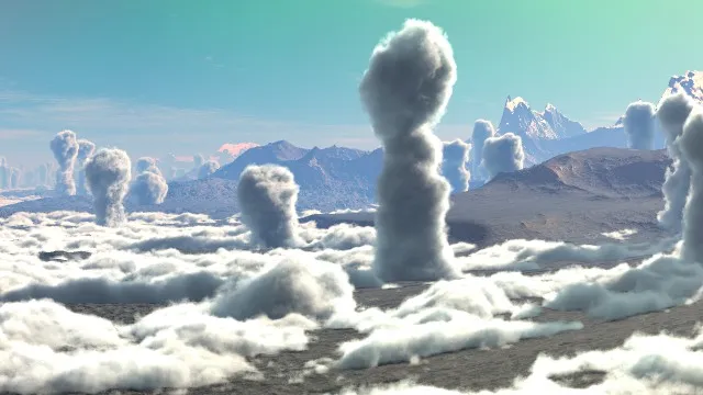
Mushroom Clouds

---

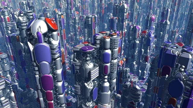
Opaque + Light

Combines Opaque mode with Volumetric Light mode. See above. The volumetric light has to be provided by a second output of the ArtMatic file. Opaque + Light is suited to creating lamps, illuminated cities, and special effects such as light rays or reactor exhausts coming out of a spaceship.

To obtain a lamp that casts shadows, add an extra output to set the light direction. Usually, the coordinates of the source are enough to set a point-light direction, as the vector is normalised by Voyager. For a parallel light, use a constant vector.

With volumetric light casting real light, you can have ‘Opaque + Light’ lamps that can be manipulated as a single object.

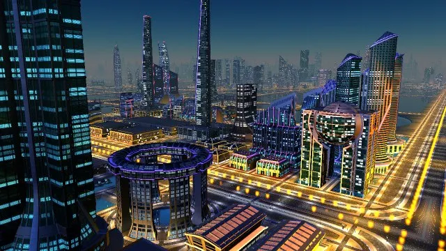
Utopia city combined with a DF lights field.

Opaque + Transparent

Combines Opaque mode with Volumetric Transparent mode. See above. The transparent volume has to be provided by a second output of the ArtMatic file. Like the other multi-mode, this mode requires an ArtMatic system that has two sets of outputs: one for an opaque object and one for a transparent object. The second object is interpreted as a transparent and reflective object. It can be coloured, but light is not accumulated volumetrically. True reflections are disabled for the opaque part, so they apply only to the transparent parts. This mode is particularly useful for creating objects that have windows in architectural design.

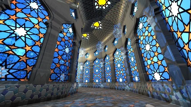
Stained glass aisle.

Opaque + Transmissive

Combines Transmissive (Surface) mode with Opaque in the same way as Opaque + Transparent for 2-output DF ArtMatic systems. The first output provides the opaque parts, and the second output provides the transparent parts.

Opaque + Transparent does not perform true refraction and is faster in all cases. True reflections are disabled for the opaque part, so they apply only to the transmissive parts. Note that ArtMatic 1.2 has a new global RGBA shader to visualise 2-output RGBA systems where A is the distance field estimate (DF).

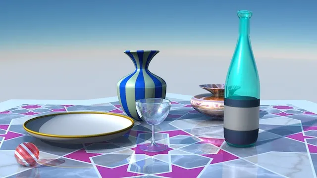
Transmissive glass and bottle.

Ambient Occlusion

Ambient Occlusion AO approximates how much light coming from the environment is blocked by the object in addition to true shadows. It provides a kind of clarity and realism not possible without it, especially when directional sunlight is absent, as in overcast sky situations. When rendering rough textured terrains or fractal objects, Ambient Occlusion is especially helpful for bringing out scene details.

Ambient Occlusion estimates the amount of non-directional ambient light that reaches various areas, as opposed to shadows caused by directional light. AO is independent of the main light direction.

Concave or hard-to-access areas are darkened. It can be applied to terrains and objects independently. Ambient Occlusion affects ambient and diffuse lighting, but not specular and reflective light channels, because it mostly simulates the blocking of light coming from any direction, not light hitting the surface from a single direction.

• Ambient Occlusion can take some time to compute and is set to OFF in Draft mode.
• DF objects provide several algorithms for Ambient Occlusion. Low-frequency AO is the most accurate but also the slowest.
• There is a global preference for AO Radius in the main Preferences dialog, but each object in a scene can have its own AO Amount setting.
• AO Amount - When AO Amount is less than 100%, only convex surfaces are affected. Amounts greater than 100% tend to affect all areas but may leave convex areas intact.
• AO Radius Preference:. Voyager scenes can have varied needs. Preferences contains a global control for the Ambient Occlusion Radius that allows you to adjust AO for the scene’s context. On a landscape dominated by large-scale features, a size of 50 metres or so will give good results. Changing the radius influences features of a certain size or detail. The same object can look quite different with different settings, so it is worth experimenting to find the setting that gives you the results you prefer.

Ideally, AO would be scale-independent, but this is currently impractical because of the enormous impact it would have on render time. Therefore, AO radius is scaled by the DF object scale when below and above 100%. This allows the same scene to have a 40-metre AO radius for terrains and large DF structures, while still having correct AO for a small 20 cm object in the foreground.

Here is an example of a fractal DF object entirely shaded by Ambient Occlusion.

---

Using Extra Outputs

When an ArtMatic DF object has one or more extra outputs, the extra output can be mapped to various shading properties such as wetness, self-illumination, or reflectivity. Using extra outputs, or X-outs for short, to modulate texture shading can greatly enhance realism and visual complexity. For example, you may have a model that provides a texture for daylight and a texture for night in an X-out channel. Turning on the channel by selecting “Self illumination” is easy, and you will typically do it for night renderings without having to change the model itself.

The extra output can be mapped to:

• ‘Nothing’: the way to turn off a particular shading option.

• ‘Self illumination’: Unlike ‘Ambient & Wetness’, which sets the amount of diffuse reflection coming from the environment, ‘Self illumination’ adds its own light to the scene, giving the impression of a luminous object. The self-illumination light colour is the X-out colour, or white if the X-out is scalar.

• ‘Wetness level’: controls the specular amount of light coming from the environment. This light can be filtered by the X-out colour, if any.

• ‘Ambient & Wetness’: controls the amount of light coming from the environment, both diffuse and specular. This light can be filtered by the X-out colour, if any.

• ‘Reflection level’: mirror reflection of light from the environment. The reflected light can be filtered by the X-out colour.

• Auto Mapping of X-out Options: The following letters placed at the end of an ArtMatic 3D DF object multi-output file cause ArtMatic Voyager to set a proper default shading option when opening or importing a new AM system. The letters can be combined in any order up to 3 letters, such as ri, wir, or wbi, when multiple X-outs are used, but a space needs to be present before them to avoid confusion with letters in the name itself.

  • i: Sets output to “Self illumination color & level”,
  • r: Sets output to “Reflection color & level”,
  • w: Sets output to “Wetness level / Specular color”,
  • b: Sets output to “Bump Map”,
  • l: 1st position - sets the first extra output to be assigned to “Volumetric Light” in the mode ‘Opaque + Light’,
  • t: 1st position - sets the first extra output to be assigned to “Transparent” in the mode ‘Opaque + Transparent’.

---

Performance Tips:

When working on a slower computer or with a particularly CPU-intensive DFRM-based scene, there may be times when making adjustments become very difficult due to the CPU being bogged down calculating the preview. This can occur while adjusting sliders and other UI elements, or simply because feedback is too slow to be practical. When this happens, there are a few tricks you can use to improve the user interface’s responsiveness.

Reduce Render Quality

The first thing to try is setting the Render Quality setting to Draft or Good. In some cases, working at a reduced quality setting until final render, can provide a noticeable improvement.

“Draft mode” cuts out extra rays and should be used initially whilst setting up a scene and positioning elements. Rendering using Best or Sublime quality is very slow and uneeded much of the time. There are many cases where a Good or Better quality render is almost indistinguishable from Best or Sublime render settings The lower-quality render can take 1/10th the time.

Deactivate Objects Temporarily

Reflective, transmissive and/or fractal objects can make CPU usage very high. Deactivating an object within the ArtMatic Object Inspector can help. Whilst inactive, adjustments may be made, for instance, sun position, camera position etc. After editing the object can be made active again. You may also temporarily turn off all reflections by setting quality to Draft mode.

Separate Texture Computation

Finding the intersection between the ray and the object is the most CPU-intensive task with DF objects, especially if the object field is poorly convergent. Texture computation is not necessary at this stage and should be put in a CT (Compiled Tree) set with Compute Only for Colors.

Sometimes the texture algorithm is much more complex than an object volume function. It may be preferrable not to compute every sample along the ray (whilst it is needed only for object shading). For constant-coloured objects or simple and fast coloured textures, it may not be worth doing this (as there is a small overhead when using a CT).

Temporarily change the Sky Mode

If your scene uses objects and volumetric skies or the Volumetric Light sky mode, you may want to temporarily set the Sky Mode to Clear Sky or Cloudy Sky. Volumetric clouds and volumetric lights can be very CPU-intensive.

Turn off shadows / ambient occlusion

The Cast Shadows option can dramatically increase calculation time. In some cases, this option can increase rendering time by as much as a factor of 10. Turn it off until you need it. If you are rendering animation, render some test frames to see if the option is worth the added rendering time. Ambient Occlusion can be set to None for each object, or globally bypassed in Draft render mode.

---

Troubleshooting DF Objects:

Object invisible:

Ensure the object is not below ground, too small, or outside the camera’s range.

Object artefacts:

Artefacts in rendering or shadows usually mean the DF field is inaccurate and convergence is poor. Revise the maths of the field, or lower the field amplitude to make convergence safer.

Black screen:

The camera is probably within the object. To fix this, move the camera outside the object’s bounds. Otherwise, the field may no longer have any “outside”, meaning negative values that define an empty region around the object. Revise the maths of the field to ensure it does have an “outside”.